
Accurate, localized rain prediction is critical for agriculture, disaster preparedness, and urban planning. The current standard is bifurcated by economic status.
Developed nations run networks of Doppler radar installations — each costing between $300,000 and $1,000,000+ — backed by supercomputer clusters solving fluid dynamics equations to simulate the atmosphere at scale (ECMWF, GFS global models). In contrast, large parts of the developing world and many rural regions lack radar coverage entirely. Farmers, local planners, and disaster managers in these areas fall back on coarse global models that fail to capture local microclimates, or on nothing at all.
The Jezreel Valley sits in one of these blind spots. Flanked by Mount Carmel to the west, the Galilee highlands to the north, and the Gilboa ridge to the southeast, the valley has a distinct precipitation microclimate driven by orographic channeling and Mediterranean sea-breeze dynamics — effects that global models handle poorly at the local scale.
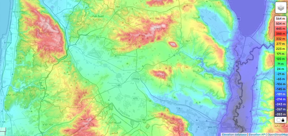
The gap is not a data problem — cheap commercial weather stations cost $2,000–$5,000 each, orders of magnitude cheaper than radar. The gap is an algorithmic one: existing methods for turning sparse point observations into a continuous weather surface either require expensive compute (Numerical Weather Prediction) or make assumptions that break down in complex terrain (Kriging assumes spatial uniformity, which the North District of Israel violates badly due to its varied topography).
This system addresses that gap by combining two ML models. Kriging — the standard geostatistical interpolation algorithm — was evaluated and rejected on two grounds: it assumes spatial uniformity (stationarity), which the North District's varied terrain violates, and it requires inverting an n×n covariance matrix at O(n³) cost upfront, and O(n²) per prediction thereafter — compared to tree-based inference which runs in O(M × d) where M and d are fixed after training, making each prediction effectively constant time.
The result is a virtual radar — localized hourly nowcasts and short-range forecasts for 1,271 grid cells across the valley at ~0.935 km spacing, with no radar infrastructure required.
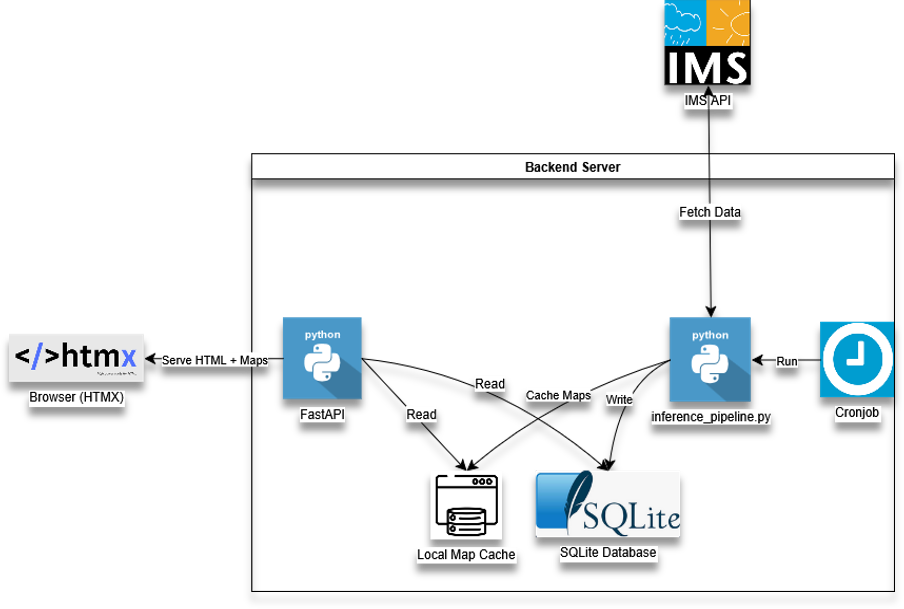
Every hour, a cronjob triggers the inference pipeline, which fetches the last 48 hours of observations from 19 weather stations operated by the Israel Meteorological Service (IMS) via their public API. Stations cover the Jezreel Valley and include coastal reference stations in Haifa and Tel Aviv. Each fetch retries up to 5 times with 30-second backoff on network failure.
The IMS delivers data at 10-minute intervals. The pipeline aggregates these into complete 1-hour windows — summing rainfall, averaging wind and humidity, and taking max/min for temperature extremes. Only complete hours are stored.
Fetching the last 48 hours on every run (rather than just the last hour) provides automatic backfill: if the server goes offline and restarts, it catches up without manual intervention. Inserts are duplicate-safe.
Raw sensor data requires more than a null check. Two categories of problems were discovered and addressed:
Sentinel values: IMS rain sensors emit -59994.0
to signal a hardware outage. This is a valid number that passes standard null checks — during early
development it inflated rain RMSE from ~0.36 mm to ~203 mm before being identified. The cleaning pipeline
now rejects any rain reading below zero as NaN.
Wind vector decomposition: Wind direction is circular — averaging 0° and 360° (both north) gives 180° (due west), which is physically wrong. The pipeline decomposes wind speed and direction into Cartesian u/v vector components before aggregation. Vector averaging is mathematically correct for circular quantities.
Additional guardrails reject temperature logic violations (T_max < T_avg)
and fill short gaps of up to 2 consecutive missing hours via linear interpolation.
The cleaned station data feeds into 8 RFSI models — one per meteorological feature (rain, wind speed, wind u/v vectors, dew point, relative humidity, daily max/min dew point). Each model estimates current conditions at all 1,271 virtual grid cells across the valley.
The RFSI feature vector for each target cell includes:
Terrain features are included for rain, wind, and humidity models — TPI in particular captures orographic channeling effects (whether a cell sits in a valley, on a ridge, or on a slope), which are the dominant local driver of wind speed and precipitation distribution in the North District.
The interpolated grid state feeds into 4 independent XGBoost forecast models — one per horizon (t+1h, t+3h, t+6h, t+12h). Each model predicts per-cell rainfall intensity using a two-layer feature vector:
Four independent models avoid the error compounding of recursive multi-step prediction, where each forecast is passed back as input for the next step. Each model instead predicts directly from real observed features.
After inference, the pipeline pre-renders all 5 Folium maps (current interpolation + 4 forecast horizons) and caches them to disk as HTML files. The FastAPI server serves these cached files directly — map requests return in under 800ms. If the pipeline itself fails, the server continues serving the last successfully generated maps with their original timestamp rather than returning an error.
The key risk in spatial ML is data leakage through spatial autocorrelation: in standard k-fold cross-validation, training stations are geographically close to the test station, so the model effectively sees correlated data during training and produces overly optimistic error estimates.
To prevent this, Afula (station 16) was held out entirely from all training stages — neither as a training target nor as a neighbor for any other station during neighbor graph construction. No information from Afula could reach any model through any path during training. This is called Leave-Location-Out Cross Validation (LLOCV).
All RFSI performance numbers below reflect evaluation on this never-seen location.
The XGBoost forecast models use an 80/20 chronological train/test split — no future timestamps can leak into training. Models are evaluated on storm hours only (rain ≥ 0.1 mm/h) using RMSE and F1 score, compared against a persistence baseline (predicting the last observed value forward).
The closest grid cell to Afula station is cell 639, 0.53 km away. The full end-to-end pipeline — interpolation followed by forecasting — was validated against real Afula ground truth across approximately 47,000 hourly samples spanning 5 years.
This evaluation fully decomposes the pipeline error: the spatial interpolation RMSE (1.41 mm/h storm-only at Afula's cell) establishes the reconstruction baseline before any forecasting is applied. The gap between that and the t+1h forecast RMSE (1.637 mm/h) represents the pure cost of predicting one hour ahead on top of spatial reconstruction.
IDW (Inverse Distance Weighting) is the parameter-free baseline that weights observations by the inverse of their distance to the target.
| Feature | RFSI MAE | IDW MAE | RFSI RMSE | IDW RMSE |
|---|---|---|---|---|
| rain — mm/h (global) | 0.0432 | 0.0479 | 0.3255 | 0.3596 |
| rain — mm/h (events ≥ 0.1mm) | — | — | 1.4819 | 1.5624 |
| ws — m/s | 0.7924 | 1.1119 | 1.0042 | 1.2957 |
| td — °C | 1.2967 | 1.0182 | 1.6628 | 1.4104 |
| rh — % | 4.2538 | 4.2575 | 5.6431 | 5.8825 |
| tdmax — °C | 1.1890 | 0.9822 | 1.6070 | 1.3671 |
| tdmin — °C | 1.3368 | 1.0904 | 1.8160 | 1.5004 |
| u_vec — m/s | 0.8624 | 0.9760 | 1.1308 | 1.2184 |
| v_vec — m/s | 0.7278 | 0.7655 | 0.9352 | 1.0043 |
RFSI outperforms IDW on all precipitation and wind features. Temperature features (td, tdmax, tdmin) are spatially smooth fields where distance-weighted averaging suffices — RFSI complexity adds noise rather than signal for smooth gradients.
Evaluated on storm hours only (rain ≥ 0.1 mm/h) at cell 639, 0.53 km from Afula.
| Horizon | RMSE | Persistence RMSE | Skill vs Persistence | F1 |
|---|---|---|---|---|
| t+1h | 1.637 mm | 1.837 mm | +10.9% | 0.66 |
| t+3h | 1.748 mm | 2.018 mm | +13.4% | ~0.58 |
| t+6h | 1.708 mm | 2.072 mm | +17.6% | ~0.52 |
| t+12h | 1.740 mm | 2.134 mm | +18.5% | 0.41 |
Skill improves at longer horizons because persistence degrades faster than the model as the forecast window grows — a well-known characteristic of storm forecasting systems consistent with the atmospheric predictability limit.
 Israel Meteorological Service